How to Freeze Cells in Microsoft Excel

Microsoft Excel makes it easy to analyze and organize large scale of data. Some time when we working with large spreadsheets, we can lose track of what each column or row represents. And scrolling back to the top is a pain and causes to lose our place in the main area. The simple solution to this is to freeze cells to keep that header information and other important data always in our view.

In simple terms, when we freeze a cell, that cell will continue to display on the window even when we scroll up and down, as well as left and right. That makes it easy to visually keep track of your data and to compare data between cells.

let's see some different scenario.

Step to freeze row or column in Excel

1. Click on the View tab on the top Menu bar.
2. Select the Freeze Panes option.
3. From the dropdown menu, Select the option Freeze Top Row or Top column.

Steps to freeze rows and columns together in Excel

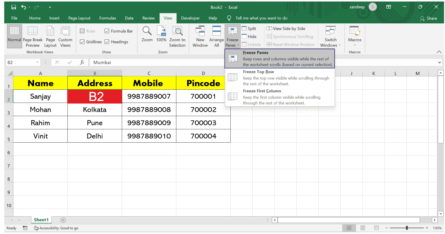
1. Select the cell below the row you wish to freeze and next to the column you want to freeze. For a example, to freeze row 1 and column A, we need to select cell B2.
2. After selecting the B2 cell, go to View tab.
3. Select the Freeze Panes option.
4. From the dropdown menu that appears, click on the Freeze Panes option.

Steps to unfreeze cells

1. Click on the View tab in menu bar
2. Select Freeze Panes option
3. Select Unfreeze Panes from the dropdown menu.

All the cell will be Unfreeze.