Vlookup Formula in Excel

Vlookup stands for Vertical Lookup. It is an Excel function that works with data in vertically arranged tables, which allows searches across columns.

It is a function that makes Excel search for a certain value in a column, in order to return a value from a different column in the same row.

Syntax of Vlookup formula in Excel

The VLOOKUP formula has 4 main components:

• Lookup Value : The value you want to find or view.
• Table Array : The Table Array or Range in which you want to find the Lookup Value and the return value
• Column Index : Number of column from which you want to get value from table array or range.
• Num (range lookup) : 0 or FALSE for an exact match with the value your are looking for; 1 or TRUE for an approximate match.


• Syntax: VLOOKUP([value], [range], [column number], [false or true])

Example of Vlookup Formula in excel

In our example we have a list of Student and their marks. We want to find the Rakesh Math number quickly in this table.

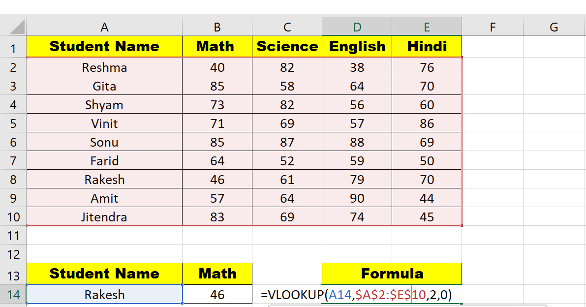
1. Type the function syntax =VLOOKUP([value], [range], [column number], [false or true])
2. Enter the lookup value, in my case it is A14 cell
3. Now enter the table_array ($A$2:$E$10)
4. Now enter the col_index_num (2)
5. Now enter the range lookup (true or 0)